When we analyze algorithms, we are interested in their correctness (they do the right things) and efficiency (they use not too much time, memory, or other resources). This post is about the running time of divide-and-conquer algorithms and one of the corner stone methods to analyze those.

For iterative algorithms, estimating the running time is often a bit easier, as we essentially only have to give upper bounds for how often a certain for or while loop is executed. For recursive algorithms this can be a lot harder (one of the most astonishing examples is the Ackermann function) but for practical purposes, there is a standard blackbox technique that allows us to bound the running time of recursive divide-and-conquer algorithms. Those have often the following very simple structure:

function divide&conquer(object O of size n):
	if n = 1:
		return solution
	d[1] = divide&conquer(divide_1(O))
	...
	d[a] = divide&conquer(divide_a(O))
	return conquer(d[1], ..., d[a])

This pseudocode above requires a bit of explaining. We have a generic divide-and-conquer algorith that operates on some object O of size \(n\), this could be for instance, the number \(n\) itself or a list of objects of length \(n\). If the object is small enough returning the solution is usually trivial, so we just do that; otherwise we recurse and split the problem up into \(a\) smaller problems that we obtain from the functions divide_k. If these subproblems have all the size \(\frac{n}{b}\) for some constant \(b\), we get a very regular looking recursion tree as below.

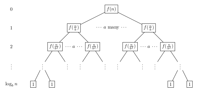
The nodes are labeled with the amount of work that needs to be done in the divide_k and the conquer method for an object of size \(\frac{n}{b^i}\) (at recursion depth \(i\), the level of the recursion tree); we denote this by a function \(f\), which we assume to be known; this is often a reasonable assumption. If we want to describe the running time of divide&conquer, we can describe this by a straight forward recursive formula:

\[T(n) = a T(\tfrac{n}{b}) + f(n) \qquad\text{and}\qquad T(1) = 1.\]

But this alone is not yet helpful. We would like to give an upper bound to some known function like \(n^2\) or \(n \log n\); here we (often) can apply the Master Theorem.

Master Theorem. Let \(T(n) = a T(\frac{n}{b}) + f(n)\).

• (i) If \(f(n) \in \mathcal{O}(n^{\log_b a - \varepsilon})\) with \(\varepsilon > 0\) then \(T(n) \in \Theta(n^{\log_b a})\).
• (ii) If \(f(n) \in \Theta(n^{\log_b a})\) then \(T(n) \in \Theta(n^{\log_b a} \log n)\).
• (iii) If \(f(n) \in \Omega(n^{\log_b a + \varepsilon})\) with \(\varepsilon > 0\) and there exists \(c < 1\) such that for all sufficiently large \(n\), \(a f(\frac{n}{b}) \leq c f(n)\) then \(T(n) \in \Theta(f(n))\).

Intuitively, the three cases of the Master Theorem correspond to the three cases how root- pr leaf-heavy the recursion tree is:

• (i) The amount of leaves (and hence, overall subproblems) is so big that it outweighs the work that has to be done in individual nodes.
• (ii) The amount of work in every level of the recursion tree is the same.
• (iii) The amount of work in the root node is so big that that it outweighs the rest of the work in the tree.

The proof of the Master Theorem is often omitted in university courses; but it is actually not so terribly hard, so here it is.

Proof. For simplicity, let us assume that \(n\) is a power of \(b\). This is reasonable as we can always pad the input such that it holds but this padding is within a factor of \(b\) (a constant), so we never have to pad a lot. The total amount of work in the tree is

\[T(n) = \underbrace{\sum_{i=0}^{\log_b n-1} a^i f(\tfrac{n}{b^i})}_{g(n)} + \underbrace{\Theta(a^{\log_b n})}_{=\Theta(n^{\log_b a})}.\]

Case (i). We have \(f(n) \in \mathcal{O}(n^{\log_b a - \varepsilon})\) with \(\varepsilon > 0\). Then this yields \(f(\frac{n}{b^i}) \in \mathcal{O}((\frac{n}{b^i})^{\log_b a - \varepsilon})\) with \(\varepsilon > 0\). Hence,

\[g(n) \in \mathcal{O}\left(\sum_{i=0}^{\log_b n-1} a^i \left(\frac{n}{b^i}\right)^{\log_b a - \varepsilon}\right).\]

The expression in the Landau-\(\mathcal{O}\) however, can be simplified:

\[\begin{aligned} \sum_{i=0}^{\log_b n-1} a^i \left(\frac{n}{b^i}\right)^{\log_b a - \varepsilon} &= n^{\log_b a - \varepsilon} \sum_{i=0}^{\log_b n-1} \left(\frac{ab^\varepsilon}{b^{\log_b a}}\right)^i\\ &= n^{\log_b a - \varepsilon} \sum_{i=0}^{\log_b n-1} (b^\varepsilon)^i\\ &= n^{\log_b a - \varepsilon} \left(\frac{b^{\varepsilon \log_b n} - 1}{b^\varepsilon - 1}\right)\\ &= n^{\log_b a - \varepsilon} \underbrace{\left(\frac{n^\varepsilon - 1}{b^\varepsilon - 1}\right)}_{\mathcal{O}(n^\varepsilon)}\\ &= n^{\log_b a}. \end{aligned}\]

Hence, in total we have \(T(n) = \mathcal{O}(n^{\log_b a}) + \Theta(n^{\log_b a}) \in \Theta(n^{\log_b a})\).

Case (ii). We have \(f(n) \in \Theta(n^{\log_b a})\) and hence, \(f(\frac{n}{b^i}) \in \Theta((\frac{n}{b^i})^{\log_b a})\) for all \(i\). Substituting this again into \(g(n)\) yields

\[g(n) \in \Theta\left(\sum_{i=0}^{\log_b n-1} a^i \left(\frac{n}{b^i}\right)^{\log_b a}\right).\]

which simplifies to

\[\begin{aligned} \sum_{i=0}^{\log_b n-1} a^i \left(\frac{n}{b^i}\right)^{\log_b a} &= n^{\log_b a} \sum_{i=0}^{\log_b n-1} \left(\frac{a}{b^{\log_b a}}\right)^i\\ &= n^{\log_b a} \sum_{i=0}^{\log_b n-1} 1\\ &= n^{\log_b a} \log_b n. \end{aligned}\]

Thus, in total we have \(T(n) = \Theta(n^{\log_b a} \log_b n) + \Theta(n^{\log_b a}) \in \Theta(n^{\log_b a} \log_b n)\).

Case (iii). Finally, we have \(f(n) \in \Omega(n^{\log_b a + \varepsilon})\) and \(a f(\frac{n}{b}) \leq c f(n)\) for some \(c < 1\). Note that \(g(n) \in \Omega(f(n))\) as \(g(n)\) contains \(f(n)\) in its definition (assuming that \(n\) is a power of \(b\) and all other terms of \(g(n)\) are also non-negative. Then we obtain

\[\begin{aligned} g(n) &= \sum_{i=0}^{\log_b n-1} a^i f(\tfrac{n}{b^i})\\ &\leq \sum_{i=0}^{\log_b n-1} c^i f(n)\\ &\leq f(n) \sum_{i=0}^{\infty} c^i\\ &= f(n) \tfrac{1}{1-c}. \end{aligned}\]

Hence \(g(n) \in \mathcal{O}(f(n))\) and together with the leaf-term we obtain \(T(n) = \Theta(f(n)) + \Theta(n^{\log_b a}) \in \Theta(f(n))\).